Numerical analysis · Coursework report

Δt ≤ h/c is not enough

A sharp stability analysis of P1 finite elements + leapfrog for the one-dimensional wave equation. Computing the spectrum of the pair (S, T) in closed form turns the usual sufficient CFL guess into a necessary and sufficient condition — and shows that the consistent mass matrix needs a step √3 times smaller than the textbook bound suggests.

Course report, Numerical Analysis for PDEs — Faculty of Mathematics and Computer Science, VNU-HCM University of Science · 29 July 2026
Written with Nông Thanh Toàn · 19 pages, Vietnamese

Read the report (PDF, VI) Code & verification

The result

1/√3

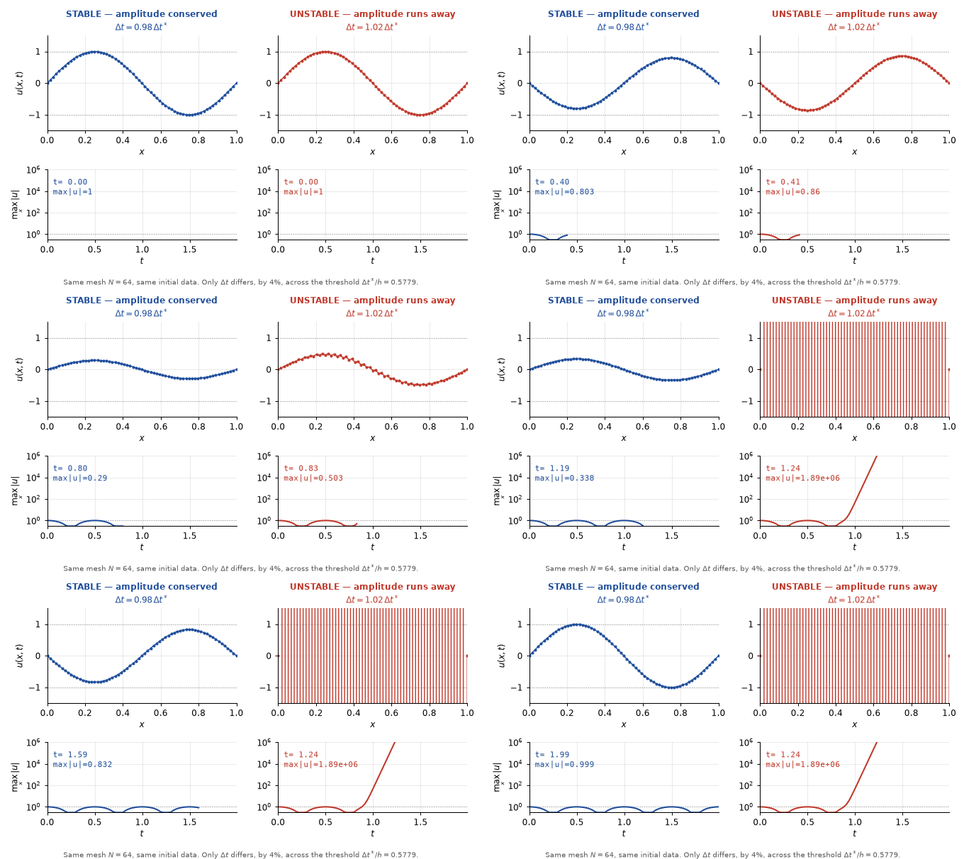
Exact CFL constant for the consistent mass matrix (θ* = Δt/h = 0.5774), against the 1.0 the familiar bound implies.

4 s.f.

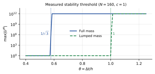
Agreement between the analytic threshold and the measured one — the sweep flips at 0.5776 for N = 160, predicted 0.577434.

2.00 / 1.00

Observed convergence orders in the L² norm and the H¹ semi-norm, over six mesh refinements from N = 10 to N = 320.

4 / 4

Tables in the report recomputed from source and checked digit-for-digit by a script that fails the build on a mismatch.

The bound is sharp, from both sides. Same mesh (N = 64), same initial data, same solver — only Δt differs, and only by 4%. At 0.98 Δt* the amplitude is conserved to within 1%; at 1.02 Δt* it passes 10⁶ before t = 1.3, and the run is cut off there. A demonstration from one side only could not tell a sharp bound from any tighter one, which is why both are shown. The trace underneath is max_x|u| on a log axis, so the growth is visible over six decades; both panels share one time axis, so the unstable run visibly stops where it diverges.

The one-line version. Stability of the leapfrog scheme is governed by the largest generalised eigenvalue of the stiffness/mass pair, and for P1 elements that eigenvalue is known exactly. Full mass matrix: λ_max → 12/h², so Δt < h/(c√3). Lumped: λ_max → 4/h², so Δt < h/c. Same mesh, same order of accuracy, step sizes a factor of 1.73 apart.

The problem

The model problem is the homogeneous Dirichlet wave equation on the unit interval: find u(x,t) with u_tt − c²u_xx = 0 on (0,1) × (0,T), u(0,t) = u(1,t) = 0, and given initial displacement and velocity. Discretise in space with piecewise-linear P1 elements and in time with the centred (leapfrog) difference, and you get the three-term recursion that every course covers.

What courses usually do not pin down is the stability limit. The bound quoted from the finite-difference case, Δt ≤ h/c, is presented as if it carried over. It does not. Run leapfrog with a consistent mass matrix at Δt = 0.9h/c and it diverges — quietly at first, because the unstable mode is the highest one and typical initial data barely excites it, then catastrophically.

So the question this report answers is the sharp one: for which Δt is the scheme stable, exactly — not "for which Δt can we prove it is stable".

The analysis

Eliminating the boundary degrees of freedom keeps the semi-discrete system symmetric, T Ü + c² S U = 0, with T the mass matrix and S the stiffness matrix — both symmetric positive definite and tridiagonal. Expanding in the generalised eigenvectors of (S, T) decouples the recursion into scalar three-term recursions, one per mode, and each is stable exactly when its amplification polynomial has roots on the unit circle. That gives the condition on the step directly:

Δt < 2 / (c · √λ_max(T⁻¹S)) necessary and sufficient — not just sufficient

The step that makes this sharp rather than decorative is that λ_max is available in closed form on a uniform mesh, for both choices of mass matrix. Writing θ_m = mπ/N:

Closed-form spectra and the CFL constants they imply. (swipe the table sideways)

Mass matrix	λ_max	h → 0	CFL bound	θ* = Δt/h
Full (consistent)	(6/h²)·max (1−cos θ_m)/(2+cos θ_m)	12/h²	Δt < h/(c√3)	0.5774
Lumped	(2/h²)·max (1−cos θ_m)	4/h²	Δt < h/c	1.0000

That is the whole explanation for the failure above. Δt ≤ h/c is the lumped constant; applying it to the consistent mass matrix overshoots the true limit by √3. The report also proves the matching convergence result via the Ritz projection — which avoids an uncontrolled remainder term and removes any need for the Aubin–Nitsche lemma — giving O(h²) in L² and O(h) in the H¹ semi-norm for P1.

Numerical evidence

Four experiments, all against the exact solution u(x,t) = cos(2πct)·sin(2πx), errors measured at T = 1 with 5-point Gauss–Legendre quadrature per element. Every number below was regenerated from source for this page.

1 — Spatial order

Full mass matrix, θ = Δt/h = 0.5, measured at T = 1. Order estimated by p ≈ log₂(E(h)/E(h/2)). (swipe the table sideways)

N	h	Δt	‖u−Û‖_L²	order	\|u−Û\|_H¹	order
10	0.100000	0.050000	3.0679e−02	—	8.0145e−01	—
20	0.050000	0.025000	6.6945e−03	2.20	4.0227e−01	0.99
40	0.025000	0.012500	1.6129e−03	2.05	2.0138e−01	1.00
80	0.012500	0.006250	3.9944e−04	2.01	1.0072e−01	1.00
160	0.006250	0.003125	9.9623e−05	2.00	5.0364e−02	1.00
320	0.003125	0.001563	2.4891e−05	2.00	2.5183e−02	1.00

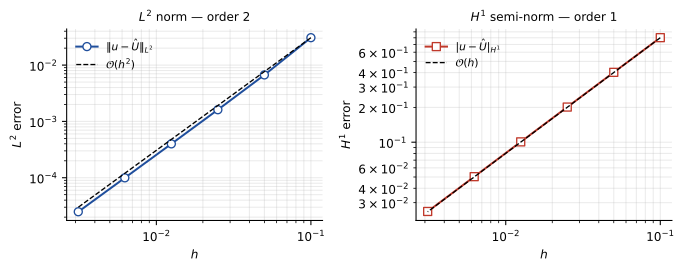
Two log–log plots of error against mesh size h. The L² error follows a slope-2 reference line and the H¹ semi-norm follows a slope-1 line across all six refinements. — Errors against `h` on log–log axes, with O(h²) and O(h) reference lines. The data run parallel to the references over the whole range.

Animation, two panels of the same run. Left, the first two periods: the computed solution sits on the exact one. Right, eighteen periods later: both still reach the same peaks, but they are visibly out of step with each other. — The scheme running (N = 20, θ = 0.5), the same solve shown at two epochs. Early, the two curves are indistinguishable. 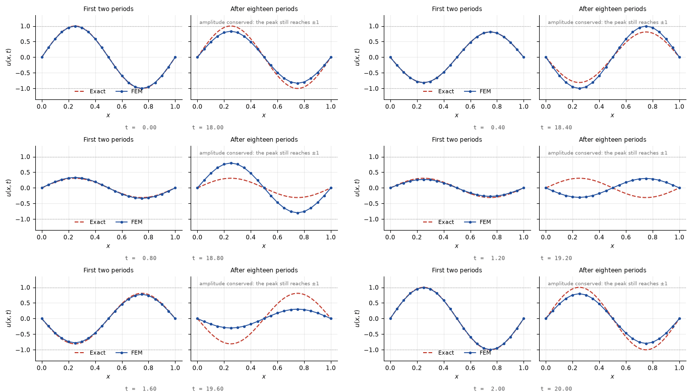Eighteen periods later they are visibly out of step — and the dotted guides show why that is *dispersion, not decay*: the peak over the late window is `1.000000` against `0.999869` over the early one, so the amplitude is conserved and the error is entirely in the phase, exactly as the discrete energy identity predicts. 41 frames, one every second time step — computed states throughout, never interpolated.

2 — Temporal order

To separate the time error from the space error, N is held at 200 and successive halvings of Δt are compared Richardson-style: ‖Û_Δt − Û_Δt/2‖ has the same order as the temporal error.

N = 200 fixed, T = 1. (swipe the table sideways)

θ = Δt/h	Δt	‖Û_Δt − Û_Δt/2‖_L²	order
0.500000	2.500e−03	1.023662e−08	—
0.250000	1.250e−03	2.299690e−09	2.15
0.125000	6.250e−04	5.586810e−10	2.04
0.062500	3.125e−04	1.386980e−10	2.01
0.031250	1.563e−04	3.466993e−11	2.00

Order 2 confirms the analysis and, with it, the second-order initialisation of the first time step — a first-order start would have shown up here as a degraded order.

3 — Locating the threshold

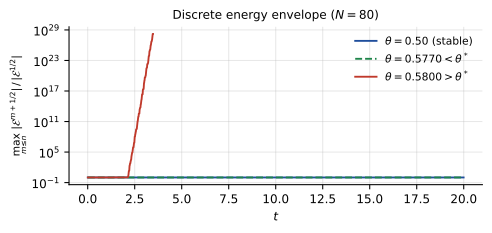
The direct test of the sharp condition: sweep θ = Δt/h and record the amplitude after M = ⌊T/Δt⌋ steps from data normalised to 1. The highest mode is seeded at amplitude 1e−8 so that an instability shows up immediately instead of waiting for round-off to grow it.

Amplitude max|U^M|, full mass matrix. Analytic thresholds: θ*(N=80) = 0.577684, θ*(N=160) = 0.577434; the h → 0 limit is 1/√3 = 0.577350. (swipe the table sideways)

θ	N = 80	N = 160	State
0.5700	9.999e−01	9.999e−01	both stable
0.5774	9.997e−01	1.000e+00	both stable
0.5776	9.998e−01	1.002e+00	N = 160 just past its threshold
0.5778	9.998e−01	2.362e+00	N = 160 diverges
0.5780	9.999e−01	2.065e+02	N = 160 diverges
0.5800	2.242e+02	1.623e+14	both diverge

The measured threshold matches θ* to four significant figures. The detail worth noticing is the row at θ = 0.5776, where N = 160 has gone unstable while N = 80 is still fine — exactly what the closed form predicts, since θ* decreases with N towards 1/√3 from above. A coarse-mesh test would have passed here and shipped the bug.

Semi-log plot of final amplitude against θ. Two near-vertical walls: the full-mass curve turns up at θ ≈ 0.577 and the lumped-mass curve at θ = 1. — Amplitude against θ = Δt/h at N = 160. Two vertical walls, at 1/√3 for the full mass matrix and at 1 for the lumped one — the whole analysis in one picture. Past its wall each curve reaches 10¹⁴⁸, so both are capped at 10¹² for display; the flat tops are the cap, not a plateau.

Semi-log plot of normalised discrete energy over 20 time units for three step sizes. Two curves stay flat at 1; the one above the threshold grows exponentially by many orders of magnitude. — Running maximum of the normalised discrete energy (N = 80). Below the threshold it is conserved to machine precision over 20 time units — the two stable curves agree to 5×10⁻¹⁵, which is why one is dashed; **0.4% above it**, the energy grows exponentially. The envelope rather than the raw ratio, because once the scheme goes unstable the dominant mode flips sign each step and the energy passes exactly through zero, which a log axis cannot draw.

4 — What lumping buys

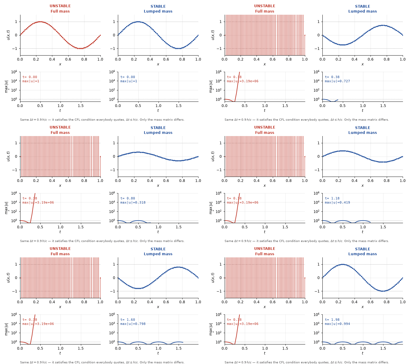
Why the familiar condition is not enough. Both panels run at Δt = 0.9 h/c, which satisfies the CFL condition everybody quotes, Δt ≤ h/c. Same mesh, same data, same step: only the mass matrix differs. The consistent mass matrix passes 10⁶ before t = 0.4 — six orders of magnitude — while the lumped one holds max_x|u| within 1% of 1 all the way to t = 2. This single step size sits between the two thresholds — above 1/√3, below 1 — which is exactly the gap the analysis is about.

Repeating experiment 1 with the lumped mass matrix at θ = 0.9 — beyond the full matrix's threshold, inside the lumped one's:

Lumped mass matrix, θ = 0.9 — an 80% larger time step than the θ = 0.5 run above, and 56% past the full matrix’s own threshold. Still stable. (swipe the table sideways)

N	h	‖u−Û‖_L²	order	\|u−Û\|_H¹	order
10	0.100000	2.5370e−02	—	8.0057e−01	—
20	0.050000	6.3636e−03	2.00	4.0226e−01	0.99
40	0.025000	1.5922e−03	2.00	2.0138e−01	1.00
80	0.012500	3.9815e−04	2.00	1.0072e−01	1.00
160	0.006250	9.9542e−05	2.00	5.0364e−02	1.00
320	0.003125	2.4886e−05	2.00	2.5183e−02	1.00

Lumping keeps the O(h²) order, gives a marginally smaller L² error, allows a step √3 ≈ 1.73 times larger, and reduces each solve to a scalar division instead of a tridiagonal solve. For this problem it wins on every axis at once — which is worth saying plainly, because mass lumping is usually introduced as a trade-off.

Reproducibility

A report whose tables cannot be regenerated is a claim, not a result. So the repository carries reproduce_tables.py: it recomputes all four tables from fem_wave.py, compares each entry against the value printed in the PDF, and exits non-zero on any mismatch.

pip install numpy matplotlib

python3 reproduce_tables.py    # recomputes Tables 1-4, checks them, writes results/tables.md
python3 make_figs.py           # figures/*.pdf  - the report's figures
python3 make_figs.py --web     # docs/fem-wave/figures/*.svg - this page's figures

Current state: all four tables agree with the report to every printed digit, and the figures on this page are generated by the same script that generates the report's, from the same computed arrays — so the page cannot drift away from the paper.

The gap it caught

The first run reproduced Tables 1, 2 and 4 exactly and failed on Table 3: the stability sweep stayed bounded at θ = 0.578 and θ = 0.580, where the report records divergence. The cause was not the analysis but the listing. Section 7.3 seeds the highest eigenmode at amplitude 1e−8 so the instability is visible at once; the growth() function printed in Appendix A did not do it. Initial data sin(2πx) contains almost none of mode m = N−1, so without the seed you are waiting on round-off.

growth() now takes seed=1e-8 (seed=0.0 restores the old behaviour) and all six rows of Table 3 reproduce to four digits. The appendix includes the file with \lstinputlisting, so the report picks up the fix on its next compile. Worth stating rather than quietly patching: the published numbers were right, the published code could not produce them, and only running it found that out.

Where it stops

One space dimension, uniform mesh, constant wave speed, homogeneous Dirichlet data, P1 elements, explicit leapfrog. The sharp constant is exact under those assumptions and claims nothing outside them.
A variable coefficient, a non-uniform mesh, or higher-order elements each change λ_max, so the constant would have to be recomputed. The method — diagonalise (S, T), read off the bound — carries over; the number does not.
The scheme is conservative but dispersive: amplitude is preserved indefinitely, phase is not. Over 20 periods at N = 20 the visible error is entirely phase lag, and no stability result improves that — it takes a finer mesh or a higher-order element.
The convergence proof is for smooth solutions. Rough initial data reduces the observed order and is not tested here.