Who I am

Map of Việt Nam, including the Hoàng Sa (Paracel) and Trường Sa (Spratly) archipelagos, with an arrow from my avatar to Hồ Chí Minh City Hoàng Sa Trường Sa TP. Hồ Chí Minh
  • NowOpen to Machine Learning / AI Engineer internships
  • StudyMathematics & Computer Science, VNU-HCM University of Science

Portfolio

Nguyễn Hoàng Tú

Machine Learning Engineer / AI Engineer

Mathematics and Computer Science undergraduate. I build machine learning systems end to end — framing the decision the model has to support, auditing the data for leakage, building a baseline before reaching for a model, and reporting what held up out of sample.

Nguyễn Hoàng Tú, Ho Chi Minh City

01 Background

About

Mathematics and Computer Science, undergraduate — VNU-HCM University of Science Expected graduation October 2027

The other half of my work is numerical analysis: solvers whose error is measured against an exact solution, and published results a script has to be able to regenerate. Both halves come down to one habit — not trusting a number until something independent checks it.

Faculty of Mathematics and Computer Science. Probability, statistics and linear algebra are the part of ML I lean on hardest — evaluation design, what a metric is actually measuring, and when a difference between two models is not a difference. The numerical-analysis side comes from three courses whose reports and code are the projects below: numerical analysis for ODEs, for PDEs, and the finite-volume topic course. Graduate of the FlyRank machine learning internship track, of which the ranking capstone was the final deliverable.

8 public repositories — five of them re-verify their results in CI on every push

02 Work

Selected Projects

Six in full, each told the same way: problem, why it matters, method, the mathematics, experiment, result, limitation — and two more below. All eight have public code; five run CI that recomputes their published numbers on every push.

Search-Ranking Refresh Queue

Flagship Paper + code public

An editorial team can review about 50 pages a week out of 18,000. The useful question is not "which pages are bad" but which pages should be opened first — an ordering problem, not a threshold one.

Why it matters
Review time is the constraint. Ordered by the model, roughly 44 of the first 50 pages opened are real decliners, against about 31 for an unordered list — the difference is a week of editorial work spent where it is needed.
Method
Defined the decision, the label and the decision point first · leakage audit that removed every window-spanning column · 24 decision-time features · a transparent rule baseline before any model · logistic regression and random forest · precision@K at the team's real capacity · client-clustered bootstrap, permutation test and calibration check · permutation importance.
Formulation
One 90-day snapshot split into three exact 30-day windows. The label is a >20% fall in impressions in the last window; every feature is knowable at the end of the second. Pages are ranked by predicted probability and scored where the team works — the top 50. P(decline∣x)=σ ⁣(w⊤x+b)precision@K=∣ top-K∩decliners ∣K,K=50\begin{gathered}P(\text{decline}\mid x)=\sigma\!\left(w^{\top}x+b\right)\\[3pt]\text{precision@}K=\frac{\lvert\,\text{top-}K\cap\text{decliners}\,\rvert}{K},\qquad K=50\end{gathered}
Experiment
30,000-row anonymised snapshot → 18,010 pages above a 100-impression floor, 30 clients. Rule, logistic regression and random forest scored out-of-fold under GroupKFold(5) by client, so no client is ever in both train and test; stability checked across five client holdouts; a deliberately leaky model kept as a control.
Result
Logistic regression on honest features: PR-AUC 0.718, precision@50 0.88 — against 0.668 / 0.74 for the rule baseline and 0.617 for random ordering, on a 0.62 base rate. The grouped split scored 0.042 lower than a naive random-row split — the split design, not the model, was doing the honest work. The leaky model reached a perfect 1.000 and was discarded. Then the result was attacked: a whole-pipeline permutation test puts chance at p = 0.005, and the model beats the rule inside 14 of 18 clients — while a client-clustered bootstrap shows the top-50 margin alone sits within noise, so it is reported as a point estimate, not a guarantee.
Limitation
One snapshot, not a time series: nothing tests whether the ranking holds across months. Thirty clients is a small sample — PR-AUC moves between 0.63 and 0.70 depending on which clients are held out. Search position and content freshness had to be dropped because they span the outcome window. No experiment, no control group: this cannot say that refreshing a page recovers its traffic.
My role
Started from FlyRank's internship starter repository — an anonymised dataset, a skeleton script and empty notebooks. The framing, the audit, the features, the models, the evaluation, the 18,010-row action queue and the paper are mine.
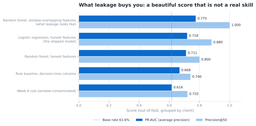
Bar chart, five models ranked by PR-AUC and precision@50 against a 61.6% base rate. The window-contaminated random forest tops it at 0.775 and a perfect 1.000; the shipped logistic regression on honest features is second at 0.718 and 0.880.
The model I threw away is the top row: with the window-overlapping columns back in, the random forest reaches a perfect precision@50 of 1.000. The shipped model is the row below it, at 0.880 — lower, and the only one of the two that means anything. Generated by capstone_pipeline.py.
Python · scikit-learn · pandas · NumPy · Matplotlib
Sharp CFL Analysis — FEM for the Wave Equation

Report + code public

Every course quotes Δt ≤ h/c as the stability limit for explicit time-stepping on the wave equation. With a consistent mass matrix that bound is wrong, and a scheme built on it diverges — quietly, because the unstable mode is the one your initial data barely excites.

Why it matters
Explicit schemes are chosen for speed, and their step size is set from exactly this bound. At Δt = 0.9 h/c — inside the textbook limit — the consistent-mass scheme passes 10⁶ before t = 0.4, while the lumped one holds its amplitude within 1% to t = 2.
Method
Closed-form spectrum of the stiffness/mass pair · a necessary and sufficient stability condition · Ritz projection for the convergence proof · Thomas algorithm, O(N) per step · a reproduction harness that recomputes every table from source.
Mathematics
P1 elements in space, leapfrog in time. The scheme is stable exactly when c2Δt2c^2\Delta t^2 times the largest eigenvalue of M−1KM^{-1}K stays below 4, and that eigenvalue is known in closed form for each mass matrix: Mu¨+c2Ku=0stable  ⟺  c2Δt2 λmax⁡ ⁣(M−1K)≤4consistent:  λmax⁡→12h2  ⇒  Δt<hc3lumped:  λmax⁡→4h2  ⇒  Δt<hc\begin{gathered}M\ddot{u}+c^{2}Ku=0\\[3pt]\text{stable}\iff c^{2}\Delta t^{2}\,\lambda_{\max}\!\left(M^{-1}K\right)\le 4\\[3pt]\text{consistent: }\ \lambda_{\max}\to\frac{12}{h^{2}}\;\Rightarrow\;\Delta t<\frac{h}{c\sqrt{3}}\\[3pt]\text{lumped: }\ \lambda_{\max}\to\frac{4}{h^{2}}\;\Rightarrow\;\Delta t<\frac{h}{c}\end{gathered}
Experiment
The step size at 0.98 and at 1.02 of the analytic threshold on the same mesh and data; consistent against lumped mass at Δt = 0.9 h/c; convergence over six mesh refinements; the solution eighteen periods on.
Result
Two distinct CFL constants where the literature usually states one. The measured threshold matches the analytic θ* to four significant figures; convergence lands on 2.00 in L² and 1.00 in H¹. All four report tables reproduce digit-for-digit in CI — after the harness caught that the shipped code was missing the 1e-8 mode seeding the report describes.
Limitation
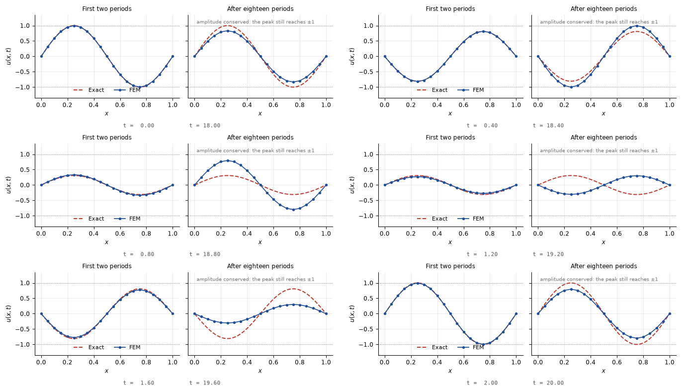
One space dimension, linear elements, a uniform mesh and homogeneous Dirichlet boundaries — the sharp constants are proved for that setting only. The scheme is stable but dispersive: eighteen periods on, the computed wave is visibly out of phase with the exact one.
My role
Two-person coursework report. The verification, the fix to the published growth() listing, and the figure pipeline that renders the report and the web page from one set of arrays are mine.
Animation, two panels of the same solve. Left, the first two periods: the computed solution sits on the exact one. Right, eighteen periods later: both still reach the same peaks but are visibly out of step.
The scheme running, the same solve at two epochs. Early the computed curve sits on the exact one; eighteen periods later they are out of step — and the peak is 1.000000 against 0.999869 early, so that is dispersion, not decay. Frames are computed states, one every second time step, never interpolated.
Python · NumPy · Matplotlib · LaTeX (XeLaTeX) · GitHub Actions

Finite-Volume Solver for the 1D Euler Equations

Package + tests public

The Euler equations grow shocks, contacts and rarefaction fans out of smooth initial data. A scheme that looks convincing on a smooth problem can be quietly wrong at a discontinuity — so the question is not whether the plot looks right, but what it is being measured against.

Why it matters
Every compressible-flow code rests on how it treats discontinuities. Without an exact reference, a misplaced shock or a smeared contact looks like a plausible curve.
Method
An exact Riemann solver as ground truth, and everything measured against it: four numerical fluxes (Lax–Friedrichs, Rusanov, HLL, HLLC) · MUSCL reconstruction with four TVD limiters and a positivity safeguard · three SSP time integrators · a CLI and a library API.
Mathematics
A conservation law for density, momentum and energy, closed by the ideal-gas law, advanced in conservative form so that shocks move at the right speed: Ut+F(U)x=0,U=(ρ, ρu, E)p=(γ−1)(E−12ρu2)Ui n+1=Ui n−ΔtΔx(Fi+12−Fi−12)\begin{gathered}U_t+F(U)_x=0,\qquad U=(\rho,\ \rho u,\ E)\\[3pt]p=(\gamma-1)\Big(E-\tfrac12\rho u^{2}\Big)\\[3pt]U_i^{\,n+1}=U_i^{\,n}-\frac{\Delta t}{\Delta x}\Big(F_{i+\frac12}-F_{i-\frac12}\Big)\end{gathered}
Experiment
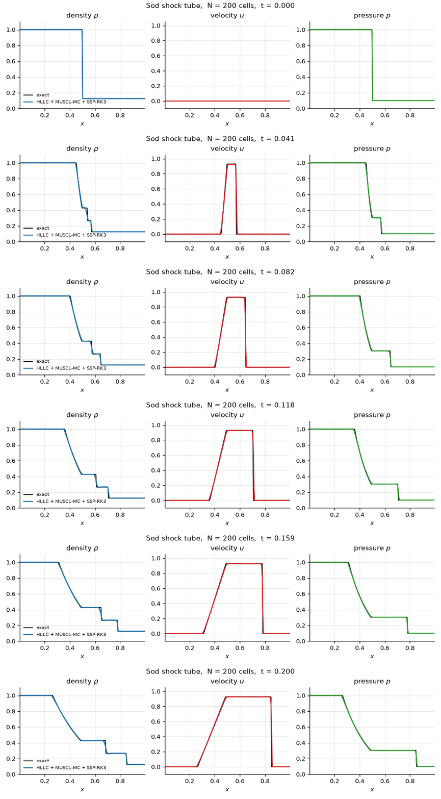
Sod's shock tube (N = 200, CFL 0.4, t = 0.2) against the exact solution for every flux; grid convergence up to N = 800; Toro's five benchmarks, including the near-vacuum 123 problem and the Woodward–Colella blast with a 10⁵ pressure ratio.
Result
The L¹ density error falls from 3.274e−02 for Lax–Friedrichs to 4.446e−03 for MUSCL–minmod — 7.4× smaller on the same grid. Observed orders 0.93–0.98 for the first-order schemes and 1.90–2.00 for the second-order ones. All five Toro problems run without tuning. 133 tests, 98% coverage, mypy clean, CI on every push.
Limitation
One space dimension. Classical Lax–Friedrichs is still climbing towards order 1 on these grids, the minmod limiter clips smooth extrema and saturates near order 1.90, and the positivity safeguard drops locally to first order wherever it acts.
My role
The repository is mine — the package, the exact solver, the test suite, the CI and the one-command path to every table and figure. The report behind it is four-person coursework (Nông Thanh Toàn, Nguyễn Hoàng Tú, Lê Minh Tuấn Kiệt, Đặng Kim Bảng), Chuyên đề giải tích số, VNU-HCM University of Science, 2025.
Three panels — density, velocity and pressure — for Sod's shock tube on 200 cells, animated in time. In each, the computed curve sits on top of the exact solution through the rarefaction fan, the contact discontinuity and the shock.
Sod's shock tube on 200 cells: density, velocity and pressure, animated in time. Black is the exact Riemann solution, colour is HLLC with MUSCL-MC reconstruction and an SSP-RK3 step — it holds the shock sharp without oscillating past it.
Python · NumPy · pytest · mypy · GitHub Actions · LaTeX

Linear Multistep Methods — Dahlquist, Derived Not Quoted

Library + tests public

Courses state the equivalence theorem — a linear multistep method converges if and only if it is consistent and zero-stable — and the BDF barrier at k ≤ 6, as facts to memorise. Both are checkable by machine, and checking them is more instructive than quoting them.

Why it matters
Every multistep ODE solver in use is a bet that this theorem holds for its coefficients. Order alone guarantees nothing: a method can be consistent to order 3 and still diverge.
Method
A library that hard-codes no conclusions. Given the coefficients it derives the order, the error constant, the roots of the characteristic polynomial, zero-stability and the absolute-stability region — so the textbook claims become test assertions the build has to satisfy.
Mathematics
A method is a pair of polynomials. Consistency and zero-stability are conditions on their roots, and Method A fails the second with a root at ζ=−5\zeta=-5: ∑j=0kαj yn+j=h∑j=0kβj fn+jρ(ζ)=∑j=0kαjζj,σ(ζ)=∑j=0kβjζjconsistent  ⟺  ρ(1)=0,  ρ′(1)=σ(1)Method A:  ρ(ζ)=ζ2+4ζ−5=(ζ−1)(ζ+5)\begin{gathered}\sum_{j=0}^{k}\alpha_j\,y_{n+j}=h\sum_{j=0}^{k}\beta_j\,f_{n+j}\\[3pt]\rho(\zeta)=\sum_{j=0}^{k}\alpha_j\zeta^{j},\qquad \sigma(\zeta)=\sum_{j=0}^{k}\beta_j\zeta^{j}\\[3pt]\text{consistent}\iff \rho(1)=0,\ \ \rho'(1)=\sigma(1)\\[3pt]\text{Method A: }\ \rho(\zeta)=\zeta^{2}+4\zeta-5\\[3pt]=(\zeta-1)(\zeta+5)\end{gathered}
Experiment
Measured order on eight zero-stable methods; BDF for k = 1 … 7; Method A on y′ = −y with h = 0.1, recomputed from its coefficients for the figure below.
Result
Measured order agrees with theory to within 0.12. BDF loses zero-stability exactly at k = 7 (max|zi| = 1.0222) — the barrier falls out of the polynomial roots instead of being assumed. Method A reaches error 10³⁷ by t = 6, multiplied by 5.3 every step. 93 tests, CI across Python 3.10–3.13.
Limitation
It makes known theorems executable; it proves nothing new. The experiments use scalar model problems such as y′ = −y rather than large systems.
My role
The library and its test suite are mine. The report is three-person coursework (L. T. Nhân, D. T. H. Yến, N. H. Tú); its 63 pages and the 50-slide deck are in the repository.
Method A: the computed solution y′ = −y with step h = 0.1. The exact solution e to the minus t stays flat near zero; the computed one flips sign every step and grows to about 10 to the 37 by t = 6. The computed solution signed log scale, sign(y)·log₁₀(1 + |y|) −1040 −1020 0 +1020 +1040 0 1 2 3 4 5 6 t exact, e−t Method A, h = 0.1 Method A: the error The error on a log axis climbs in a straight line, multiplied by 5.30 every step; it passes 1 at t = 0.9 and reaches about 10 to the 37 by t = 6. The error |Yₙ − y(tₙ)|, log scale 10−20 1 1020 1040 0 1 2 3 4 5 6 t error = 1, passed at t = 0.9 ×5.30 every step
The theorem, made concrete. This method is consistent to order 3 — higher than BDF2 — and still diverges, because its ρ polynomial has a root at z = −5: at h = 0.1 the error is multiplied by 5.3 every step. Black is the exact solution; by t = 6 the computed one has passed 10³⁷. Accuracy does not rescue a method that is not zero-stable. Recomputed from the repository's ex01_method_a.py setup.
Python · NumPy · pytest · ruff · GitHub Actions · LaTeX

Neural Networks and PINNs for Differential Equations

Thesis + code public

Physics-informed neural networks degrade on problems with a small length scale. The thesis asks why, and at which level: approximation, optimisation, or the stability of the differential problem itself.

Why it matters
PINNs are proposed as general PDE solvers, and their failures are usually reported as anecdotes. Knowing which level fails tells you what to change — the architecture, the optimiser, or the formulation.
Method
Networks studied through derivatives with respect to the input, giving explicit Jacobian and Hessian recurrences; backpropagation and forward/reverse-mode differentiation derived; gradient pathology, spectral bias and a residual-to-error stability bound, each tested by one experiment with a pass/fail criterion written down before it ran.
Mathematics
The loss is a weighted sum of mean-square residuals. For −u′′=f-u''=f on (0,1)(0,1) with the boundary condition imposed exactly, the residual bounds the error — which is why minimising it is worth doing at all: J(θ)=λrJr(θ)+λ0J0(θ)+λbJb(θ)Jr(θ)=1N∑i=1N∣rθ(xi)∣2∥eθ∥L2(0,1)  ≤  1π2 ∥rθ∥L2(0,1)\begin{gathered}J(\theta)=\lambda_r J_r(\theta)+\lambda_0 J_0(\theta)+\lambda_b J_b(\theta)\\[3pt]J_r(\theta)=\frac{1}{N}\sum_{i=1}^{N}\big\lvert r_\theta(x_i)\big\rvert^{2}\\[3pt]\lVert e_\theta\rVert_{L^{2}(0,1)}\;\le\;\frac{1}{\pi^{2}}\,\lVert r_\theta\rVert_{L^{2}(0,1)}\end{gathered}
Experiment
Six experiments on an 885-line implementation built directly on torch.autograd, no PINN library: ReLU under a second-order operator, the soft boundary constraint, spectral bias, the diffusion equation, Burgers at small viscosity, and the stability bound.
Result
Under ReLU the residual gradient is exactly 0.0; tanh reaches a 16,660× lower L² error. The operator reverses spectral bias — contradicting the thesis's own chapter 4, which the text then retracts. Diffusion to 1.0×10⁻⁴. The stability bound holds with its hypothesis (max ratio 0.0261 against 0.1013) and is exceeded up to 96× without it. 20 tests, 39 checks re-derived in CI.
Limitation
Burgers at small viscosity is a negative result: no configuration beats a relative L² error of 0.082, and adaptive weighting made it worse (0.39 and 0.35). Every problem is in one space dimension. Quantities after 4,000 Adam steps reproduce only to within 3.4% across machines, and the verification says so.
My role
Undergraduate thesis, VNU-HCM University of Science. The theory and the proofs are mine; the test suite, the verification script and the CI came later, with AI assistance, and the repository says which commits.
Plain regression: error per frequency during training Error coefficient of each frequency k = 1, 4, 8 over 8,000 Adam steps, log scale. Final values k = 1: 5.8e-05, k = 4: 1.4e-04, k = 8: 1.3e-03; relative L2 error 0.0098. Plain regression low frequency learned first · rel. L² error 0.0098 10−4 10−2 1 0 4,000 8,000 Adam steps k = 8 k = 4 k = 1 PINN residual loss: error per frequency during training Error coefficient of each frequency k = 1, 4, 8 over 8,000 Adam steps, log scale. Final values k = 1: 5.1e+00, k = 4: 1.9e+00, k = 8: 1.1e+00; relative L2 error 5.37. PINN residual loss the operator reverses the order · rel. L² error 5.4 10−4 10−2 1 0 4,000 8,000 Adam steps k = 1 k = 4 k = 8 Residual + Fourier features: error per frequency during training Error coefficient of each frequency k = 1, 4, 8 over 8,000 Adam steps, log scale. Final values k = 1: 1.5e-01, k = 4: 2.8e-02, k = 8: 1.4e-02; relative L2 error 0.109. Residual + Fourier features high frequencies first, k = 1 last · rel. L² error 0.11 10−4 10−2 1 0 4,000 8,000 Adam steps k = 1 k = 4 k = 8
The same target — sin 2πx + sin 8πx + sin 16πx, equal amplitudes — the same network and the same seed, three losses. Fit the function directly and the network learns the low frequency first: spectral bias. Train on the PDE residual instead and the second derivative weights frequency k by 4π²k², reversing the order — and that solve fails outright (relative L² error 5.4). Add Fourier features and the high frequencies converge within the first hundred steps while k = 1 is the slowest. The committed results of the thesis's experiment 3.
Python · PyTorch · NumPy · LaTeX

Inexact and Accelerated Proximal Point Algorithms

Report + code public

The accelerated proximal point method assumes each inner subproblem is solved exactly. In practice it never is — so the question is how much inexactness the O(1/k²) rate survives.

Why it matters
Every proximal step is solved approximately, by another algorithm. Güler's 1992 proof of the accelerated rate has a gap, identified by Salzo and Villa: whether acceleration survives depends on the kind of error certificate the inner solver can provide.
Method
The inexact accelerated method against the classical proximal point method under five inner-accuracy schedules, traced against the O(1/k) and O(1/k²) rates, with the convergence bound proved in the report checked numerically at every outer step.
Mathematics
The proximal operator rarely has a closed form. With inner errors shrinking as εk=O(k−q)\varepsilon_k=\mathcal{O}(k^{-q}), a type-1 certificate caps the rate at O(1/k)\mathcal{O}(1/k); a type-2 certificate keeps O(1/k2)\mathcal{O}(1/k^2) once q>3/2q>3/2: prox⁡λF(y)=arg min⁡x{F(x)+12λ∥x−y∥2}εk=O(k−q)type 1  ⇒  O(1/k),type 2, q>32  ⇒  O(1/k2)\begin{gathered}\operatorname{prox}_{\lambda F}(y)=\operatorname*{arg\,min}_{x}\Big\{F(x)+\frac{1}{2\lambda}\lVert x-y\rVert^{2}\Big\}\\[3pt]\varepsilon_k=\mathcal{O}\big(k^{-q}\big)\\[3pt]\text{type 1}\;\Rightarrow\;\mathcal{O}(1/k),\qquad \text{type 2},\ q>\tfrac32\;\Rightarrow\;\mathcal{O}\big(1/k^{2}\big)\end{gathered}
Experiment
A synthetic LASSO (n = 80, m = 30, sparsity 8); five schedules — fixed budgets of 1 and 4 inner steps, log k, √k, and exact solves — against the classical, unaccelerated method, over 121 outer steps.
Result
By k = 40 the √k schedule sits 54× below the classical method and exact solves 198×, while fixed budgets stall at 3×10⁻² and 1.4×10⁻⁴. The bound: 0 violations in 121 steps for all five schedules. 90 checks, mutation-tested — 10 planted bugs, all 10 caught.
Limitation
One synthetic instance at small scale: the experiments illustrate the theorem, they do not benchmark solvers.
My role
The repository is mine — the MATLAB and Python experiments, the build that generates the report, slides and presentation script from one set of sources, and the verification that turned the convergence bound into a CI check. The written work is group coursework (Nhóm 10), optimisation topic.
Inexact accelerated PPA on LASSO: gap per outer step F(x_k) minus F-star on log–log axes for four inner-accuracy schedules and the classical, unaccelerated method, against O(1/k) and O(1/k squared) reference rates. T_k = 1 ends at 3.2e-02; T_k = 4 ends at 1.4e-04; T_k ~ sqrt(k) ends at 3.6e-07; T_k = T_ref (exact) ends at 6.2e-09; classical PPA, not accelerated ends at 1.5e-07. Which schedules keep the rate F(xₖ) − F*, log–log 10−10 10−6 10−2 102 1 10 100 outer step k O(1/k) O(1/k²) T = 1 T = 4 √k classical exact The convergence bound, checked at every step For the square-root schedule, the actual gap F(x_k) minus F-star against the report's two bounds over 121 outer steps: it stays below both, 0 and 0 violations. The bound, checked √k schedule · 0 violations in 121 steps 10−10 10−6 10−2 102 0 40 80 120 outer step k actual gap bound, type 1 bound, type 2
Left: LASSO (n = 80, m = 30), gap to the optimum at each outer step. By k = 40 the schedules that tighten their inner solves sit far below the classical, unaccelerated method — √k by 54 times, exact solves by 198 — while fixed budgets of 1 or 4 inner steps stall at 3×10⁻² and 1.4×10⁻⁴. Right: for the √k schedule the actual gap stays under both of the report's bounds at every one of 121 steps — the check CI runs. Traces from the repository's lasso_iappa.py, whose final values match its committed summary to every digit.
MATLAB · Octave · Python · LaTeX

Other Work on GitHub

Code public

Two more public repositories: a retrieval system that shows which retriever to trust for which question, and a trading research harness built so that its answer is allowed to be "no".

Projects
  • Enterprise Hybrid RAG — question answering over PDF, DOCX and Markdown with page-level citations, built without a RAG framework: BM25 and dense retrieval, reciprocal-rank fusion, cross-encoder reranking and an abstention gate. On 50 questions over 22 documents, hybrid + reranker reaches Recall@1 0.795, against 0.585 dense-only and 0.643 BM25.
  • AI Quant Trading Research Lab — does a leakage-aware ML signal beat simple trading rules out of sample, after costs? Walk-forward refits with an embargo, logistic regression and XGBoost against buy-and-hold, momentum and moving-average baselines on SPY, QQQ, IWM, TLT and GLD, costs charged on turnover, moving-block bootstrap. A research harness: no returns are quoted, because none are committed.

03 Method

How I Approach an ML Problem

This is the order I actually work in. It is also the order in which the capstone above was built, and why its honest score is lower than its leaky one.

Define the decision first. What does someone do differently because of the output? That fixes the label, the grain and the evaluation metric — before any modelling.
Audit the data for leakage. Every feature gets checked against the decision point. Anything that spans the outcome window is dropped, however predictive it looks.
Build a transparent baseline. A rule or a simple model, scored the same way. If the model cannot beat it, the model is not the answer.
Experiment systematically. One change at a time, a fixed seed, and the same split for every candidate so the comparison means something.
Compare, then attack the result. Check stability across holdouts, inspect what the model leans on, and look for the split design that would make the number collapse.
Write down what did not work. The failures and limitations go in the report next to the results — they are what makes the results usable.

04 Toolkit

Technical Skills

Grouped by what I can actually do with them, each tied to the project where I used it.

Machine Learning
Python, scikit-learn, feature engineering, baselines, cross-validation design, precision@K and PR-AUC, leakage auditing, permutation importance
→ Search-Ranking Refresh Queue — 24 audited features, GroupKFold by client, 0.88 precision@50 vs a 0.74 rule baseline
Deep Learning
PyTorch, Transformer encoders, LSTMs, attention, training pipelines, neural ODEs and physics-informed losses
→ Neural Networks and PINNs for Differential Equations — thesis plus six experiments with committed results.
Numerical Methods and Scientific Computing
Finite element and finite volume methods, exact Riemann solvers, stability and convergence analysis, CFL conditions, mass lumping, TVD limiters, SSP integrators, LaTeX
→ Four public repositories: a sharp CFL constant matched to four significant figures, L¹ error cut 7.4× on Sod's shock tube, 133 tests at 98% coverage, and Dahlquist's barriers derived from the coefficients rather than quoted from a book
Data
pandas, NumPy, exploratory analysis, time-window design, Matplotlib
→ 30,000-row snapshot split into three exact 30-day windows; 18,010-row modelling population after an explicit filter
Engineering
Git, reproducible pipelines, fixed seeds, REST APIs, LLM integration, end-to-end testing, static deployment
→ One script reproduces the whole capstone; CI on five repositories recomputes published results on every push and fails the build on a mismatch; this page's contact form is wired to a live backend and covered by a browser test suite

05 Contact

Let’s talk.

Open to Machine Learning / AI Engineer internships. Questions about any of the work above are welcome too — this form goes straight to my inbox.